

Class D may be the future (i.e. the present), but classic AB circuits are still very much in high demand even in the hi-fi mainstream. Naturally, this invites exhaustive discussions about the technical and sonic pros and cons, but that’s not what we’re here for today. Instead, let’s get the fundamentals of this whole alphabet soup sorted: What do these “classes” even mean?
Circular sections
There is a whole range of amplifier classes, but for hi-fi applications the operating classes A, B, AB and D are particularly relevant. Let’s look at classes A and B first, as they follow a uniform basic principle: They are defined according to the proportion of the input signal over which the amplification devices (be it transistors or tubes) conduct current, where the duration of the conductivity is expressed as an angle. I know this sounds abstract, but it quickly becomes clear if we consider a sine wave as the input signal. The entire wave is analogous to a full circle, i.e. it corresponds to 360 degrees, so a half-wave “lasts” 180 degrees – there you go, duration expressed as an angle. So, if an amplification device carries current over the entire wave, it is operated with a conduction angle (also called line angle) of 360 degrees; an element that only reproduces a half-wave and is switched off during the opposite half of the wave is operated with an angle of 180 degrees. And with that we have already defined our first two classes: Class A simply means that the transistor or tube carries current permanently, while Class B describes a line angle of 180 degrees.

However, if we only allow 180 degrees to pass, we inevitably lose half of the signal – also, why not have the element conduct permanently in the first place? Since music consists of pressure peaks and dips that are electronically translated into positive and negative voltage swings, it makes sense to control an amplification element in such a way that it can modulate the voltage in both directions from the center of its operating range and thus simply track the entire signal. In fact, this is the operating principle of the technically simplest amplifier topology: single-ended amplifiers. While these are still regarded as the Holy Grail of sound quality, they unfortunately also suffer from lousy efficiency by design. After all, the amplification device works up or down from the middle of its characteristic curve, which also means that it’s permanently energized – regardless of whether a signal is present or not. As it modulates the voltage up and down from this point, it delivers, on average, exactly its full power power output, no matter if it’s idling or playing music at full blast – it’s a bit like bolting the throttle to the floor pan in a car, then controlling the speed by modulating the brakes.
Ripped apart and made whole again
For reasons of energy efficiency, it is therefore desirable to lower the base voltage from which the device swings up and down, or even set it to zero. But this means that we gain headroom for the upswing while giving up “bottom room” for the downswing, meaning that geometrically speaking, we can no longer map the entire wave to the amplification device’s characteristic. This problem can be avoided by simply splitting the signal into two half-waves and transferring them to two oppositely doped transistors (npn and pnp). This operating principle is known as push-pull amplification. Each of the transistors then only works over “its” 180 degrees of the sine wave, which brings us back to our class B. This is elegant and efficient, but comes with two drawbacks: firstly, transistors do not switch from the first millivolt, but rather have to be driven beyond a threshold voltage before they “wake up” – the signal would therefore be briefly interrupted at each transition between the wave halves, which is unacceptable in music reproduction; pure Class B amplifiers are therefore not really a thing in hi-fi.
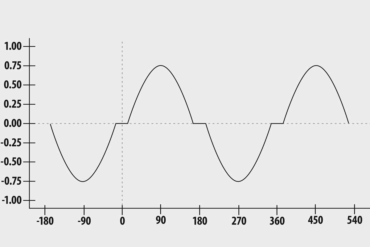
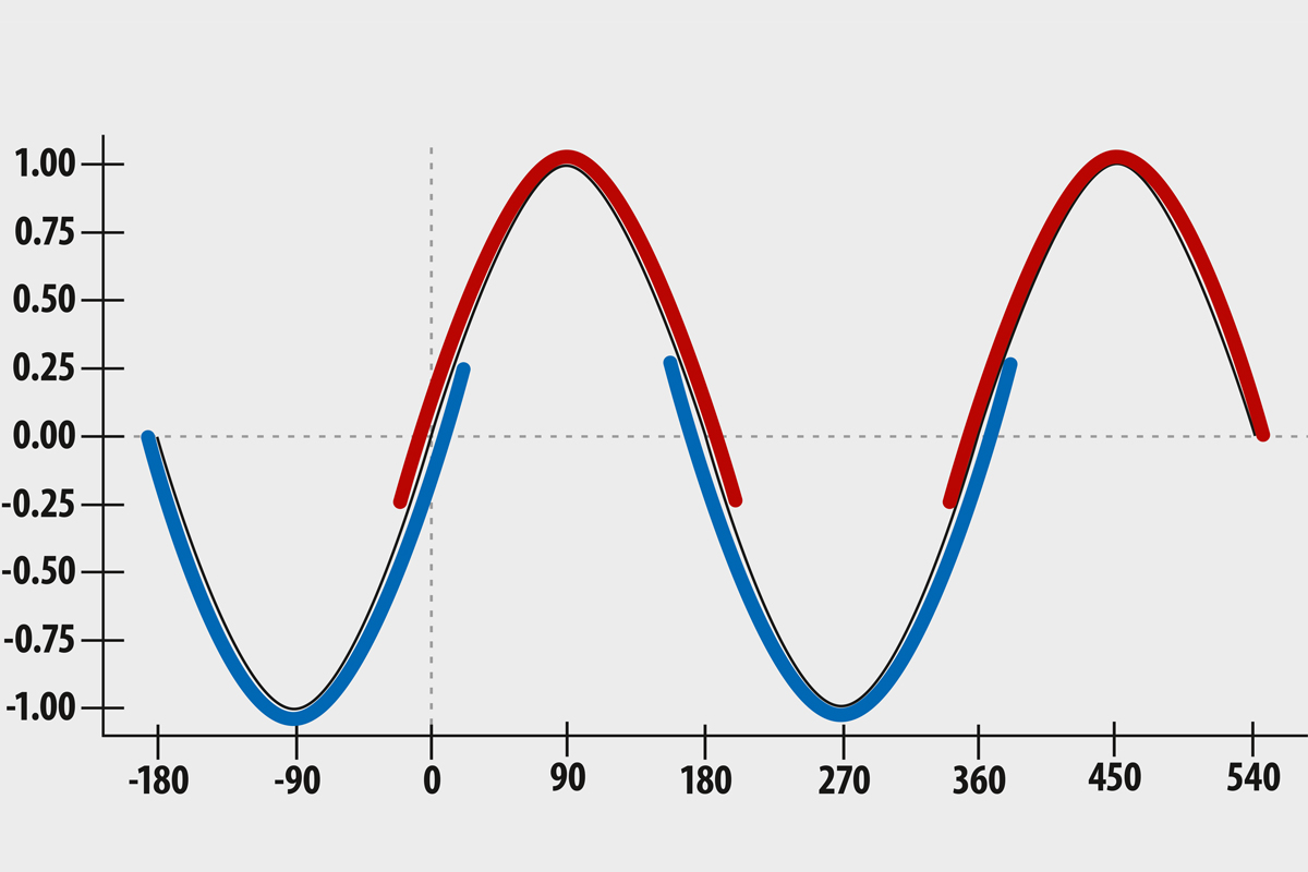
Instead, a neat little trick is used: a small quiescent current (called idle current od bias current) is applied that keeps the amplification element permanently above the threshold voltage and also enables it to transmit at least a small part of the opposite half of the wave, which increases the line angle to more than 180 degrees – and this is precisely how a Class AB circuit is defined; if the idle current is set such that both elements conduct over the full 360 degrees, we are once again talking pure Class A, even if it’s a push-pull amplifier.
Even though Class AB solves the threshold voltage issue, distortion still occurs due to the alternate switching of the amplification devices in the transition between the wave halves. As the active phases partially overlap due to the increased conduction angle, this problem only arises when the signal amplitude exceeds the bias current – below this, both amplification devices remain continuously active, and since they never switch off, no switching-related distortion occurs. In this sense, a class AB amplifier isn’t even a compromise amplifier, as it operates in actual class A at low loads and only switches to class B at higher amplitudes. In high-quality amplifiers, the idle current is therefore often set quite high so that they can deliver, say, around ten percent of their rated power in class A. This may not sound like much, but if you consider that during most of a normal listening session, less than one Watt per channel is used, such designs usually run almost continuously in Class A mode while offering plenty of power reserves for dynamic peaks.
Rounded peaks
Finally, Class D describes a completely different way of using amplification devices. Whereas the operating modes described so far modulate the conductivity of the elements between the threshold and saturation points, class D only distinguishes between on and off and usually represents the excursion curve using pulse width modulation (although pulse frequency modulation can also be used): The duration of the on versus off state over a certain period of time results in an average signal amplitude. If the switching interval is set orders of magnitude higher than the highest frequency to be reproduced – for the audio range, that would be a few hundred kilohertz, or even considerably higher – and the bandwidth is then limited to a sensible upper cut-off frequency by means of a low-pass filter, the output doesn’t “see” countless switching operations, but rather a signal amplitude that varies smoothly over time to accurately represent the amplified music signal.